
Table Of Content
Background
Automatic Cluster Gates
Applications of cluster gating
Background
Clustering is a statistical process in which events or observations from raw data are analyzed across a number of parameters and then assigned into groups called "clusters." One use case of clustering might be to take 100,000 events and assign them into 50 clusters. After the clustering, each one of those 100,000 events will belong to a cluster, and thus have an identifier of which cluster it belongs to. The identifiers will be numbers between 1 and 50. Consider this example SPADE tree with 50 nodes:
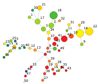
(a spade tree with 50 nodes)
If a subset of this same clustered data were visualized in a spreadsheet form:
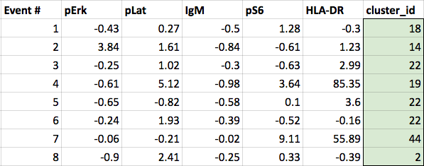
(The clustered data from the SPADE tree - a cluster_id column is added to the original data to indicate which cluster each event belongs to. This principle is the same regardless of which clustering algorithm is used.)
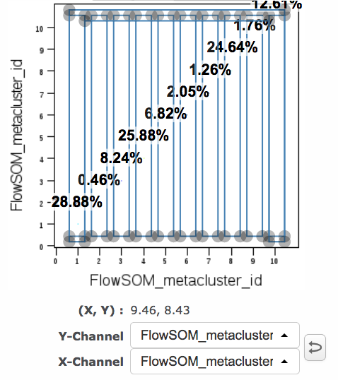
In Cytobank, if FCS files are exported from a SPADE tree (or imported from a clustering done elsewhere), the resulting files will have a cluster channel that can be used for downstream analysis. This is also the case for FCS files produced by FlowSOM and CITRUS. Plotting the cluster channel (with scales set to linear) displays the discrete cluster identifier values. These are example plots based on the SPADE tree above:
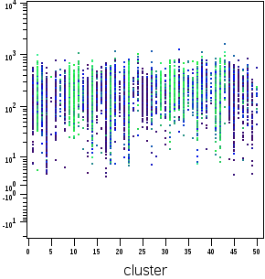
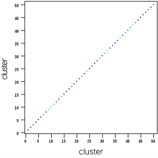
(cluster channel versus a marker) (cluster channel versus itself)
Annotation variables can be used in the same way as cluster identifiers to define groups of events or observations based on known variables. For example, in data containing one row per sample and one column per RNA transcript, you might know that some samples were given treatment 1 and some samples were given treatment 2. You can create an extra channel with this information and use it like the cluster channel described above. These annotation variables need to be coded as integers in order to be used in Cytobank. An example of how these annotation variables might be coded is shown here:
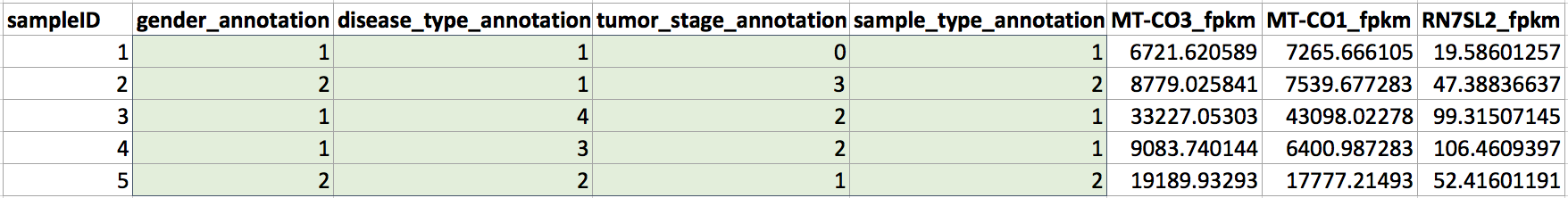
(Columns have been added for annotation variables representing gender, disease type, tumor stage, and sample type that indicate which group each sample belongs to for each of these variables. These channels can be used as cluster channels in the cluster gating workflow described below.)
Automatic Cluster Gates
Use the Automatic cluster gates functionality within the gating interface to specify groups of (meta)clusters that you want to group into one Gate/Population. You can combine ranges of (meta)clusters e.g. (1:5) and/or combinations of non-consecutive (meta)clusters e.g. (1,5,10). You cannot modify an existing gate/population’s definition in terms of (meta)cluster IDs they encompass, but you can delete ones that you want to remake as combinations of different (meta)clusters.
1) A comma-separated list of cluster ID numbers will result in the creation of gates for each number entered, one gate for each cluster.
2) You can use parentheses in the format of (1,2,3) or (6,8,10) to merge clusters. Here the number inside the bracket stands for the cluster or metacluster ID. With this formula, they are combined into a new gate showing up under Gates among all other gates. If you are combining sequential clusters such as 1, 2, and 3, you can also use (1:3) where a colon denotes a consecutive range of clusters. You can combine non-consecutive clusters using a syntax such as (1:3,10:12), which would group together clusters 1 through 3 and 10 through 12 into one gate.
(gates applied to all clusters automatically - only showing subset of clusters)
Applications of cluster gating
Visually compare clustering algorithm results
Use cluster gating in concert with colored overlay dot plots and dimensionality reduction (DR) to create a figure that show the results of DR and the results of a clustering algorithm at the same time. This is a way of visualizing the results of any clustering algorithm or multiple clustering algorithms on a DR map:
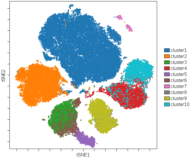
(Cluster results for a 10 node SPADE tree are colored on a viSNE plot. Both algorithms were run on the same data with the same channel selections. Areas where colors disagree show disagreements in the categorization tendency of either algorithm.)
Visually compare annotation variables with high dimensional analysis results
Use cluster gating in concert with colored overlay dot plots and DR to visualize how annotation variables are correlated with samples that are found to be similar based on DR or clustering algorithms.
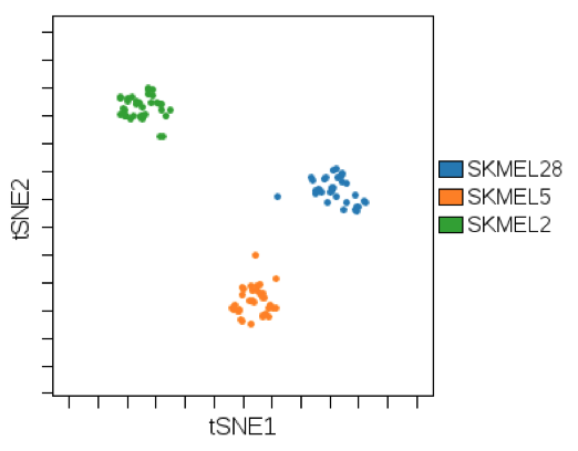
(An annotation variable representing cell line is colored on a viSNE plot. viSNE was run using multiple RNA and protein biomarkers measured in these cell lines to group similar samples. Using this coloring scheme, we can see that the biomarker expression signature across all markers is correlated with cell line.)